Lecture 13. F) Some Notes
Contents
Some Notes: Notation, z-test, t-test
[math]z_{\alpha}[/math] Notation
If you haven’t mastered the previous content, this section will be very confusing. So, please, make sure you feel well grounded, because we will now discuss other common ways in which you will see hypothesis tests written for the case of parameter [math]\mu[/math] in the normal distribution.
Consider the test [math]H_{0}:\mu=\mu_{0}[/math] vs. [math]H_{1}:\mu\lt \mu_{0}[/math], that rejects [math]H_{0}[/math] if [math]\overline{x}\lt c.[/math]
As we have seen before, the probability of a type 1 error can be calculated as
[math]\begin{aligned} & P_{\mu_{0}}\left(\overline{X}\lt c\right)\\ = & P_{\mu_{0}}\left(\frac{\overline{X}-\mu_{0}}{\frac{\sigma}{\sqrt{n}}}\lt \frac{c-\mu_{0}}{\frac{\sigma}{\sqrt{n}}}\right)\\ = & P_{\mu_{0}}\left(Z\lt \frac{c-\mu_{0}}{\frac{\sigma}{\sqrt{n}}}\right)\\ = & \Phi\left(\frac{\sqrt{n}\left(c-\mu_{0}\right)}{\sigma}\right).\end{aligned}[/math]
Above, we transformed [math]\overline{X}[/math] by subtracting its mean and dividing by its standard deviation, so that we obtain a random variable with distribution [math]N\left(0,1\right).[/math]
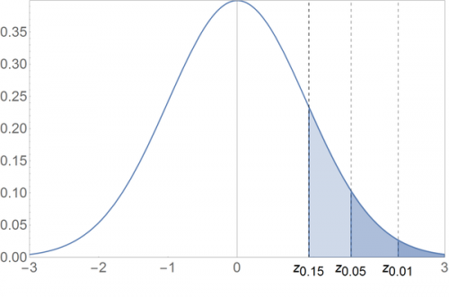
Let us define [math]z_{\alpha}[/math] implicitly, as the value of [math]z[/math] that satisfies [math]1-\Phi\left(z\right)=\alpha[/math], that is, [math]z_{\alpha}[/math] is a value s.t. a [math]N\left(0,1\right)[/math] random variable has [math]1-\alpha[/math] probability of being above it.
See the plot below for some examples:
Above, [math]z_{0.01}[/math] is given by [math]1-\Phi\left(z_{0.01}\right)=0.01\Leftrightarrow z_{0.01}=2.326[/math]. By the same procedure, [math]z_{0.05}=1.645[/math] and [math]z_{0.15}=1.036.[/math]
Also, notice that [math]z_{1-\alpha}[/math] is given by the value of [math]z[/math] that satisfies [math]\Phi\left(z\right)=\alpha[/math], and finally, because [math]N\left(0,1\right)[/math] is symmetric around zero, [math]z_{1-\alpha}=-z_{\alpha}.[/math]
Let us now solve
[math]\Phi\left(\frac{\sqrt{n}\left(c-\mu_{0}\right)}{\sigma}\right)=\alpha[/math]
with respect to [math]c.[/math]
Notice that this equality is satisfied if [math]\frac{\sqrt{n}\left(c-\mu_{0}\right)}{\sigma}=z_{1-\alpha}=-z_{\alpha}.[/math]
Solving this equation w.r.t. [math]c[/math] yields
[math]c=\mu_{0}-z_{\alpha}\frac{\sigma}{\sqrt{n}},[/math]
such that the probability of rejecting [math]H_{0}[/math] is indeed [math]\alpha.[/math]
Looking at this critical value, this means that we reject [math]H_{0}:\mu=0[/math] if
[math]\overline{X}\lt \mu_{0}-z_{\alpha}\frac{\sigma}{\sqrt{n}}.[/math]
This is an equivalent way of writing our test, which you will see in many textbooks.
The z-test: Using the Standardized Sample Mean as the Test (instead of the Sample Mean)
Up to now, we have mostly used [math]\overline{X}[/math] as the test statistic, when testing hypotheses about [math]\mu[/math], in the Normal context.
An alternative approach is to use the test statistic [math]Z=\frac{\overline{X}-\mu_{0}}{\frac{\sigma}{\sqrt{n}}}.[/math] This test statistic is the standardized sample mean, under the assumption that [math]\mu=\mu_{0}[/math].
This alternative statistic, often called the Z-score, can be useful. However, it is a priori less intuitive, because the test statistic involves a subtraction of [math]\mu[/math] under the null hypothesis. Why would we do this?
Let’s write the power function for the test:
[math]H_{0}:\mu=\mu_{0}[/math] vs. [math]H_{1}:\mu\lt \mu_{0},[/math]
using the [math]Z[/math] statistic:
[math]\beta\left(\mu\right)=P\left(reject\,H_{0}\right)=P\left(Z\lt c\right)=P\left(\frac{\overline{X}-\mu_{0}}{\frac{\sigma}{\sqrt{n}}}\lt c\right).[/math]
We appear to have a bit of a problem: the power function is supposed to depend on [math]\mu[/math]. However, [math]\mu[/math] does not show up in the expression; only [math]\mu_{0}.[/math]
We can solve this by subtracting [math]\frac{\mu}{\frac{\sigma}{\sqrt{n}}}[/math] from both sides:
[math]Pr\left(\frac{\overline{X}-\mu_{0}}{\frac{\sigma}{\sqrt{n}}}\lt c\right)=Pr\left(\frac{\overline{X}-\mu_{0}-\mu}{\frac{\sigma}{\sqrt{n}}}\lt c-\frac{\mu}{\frac{\sigma}{\sqrt{n}}}\right)=Pr\left(\frac{\overline{X}-\mu}{\frac{\sigma}{\sqrt{n}}}\lt c-\frac{\mu-\mu_{0}}{\frac{\sigma}{\sqrt{n}}}\right).[/math]
Now, the left-hand size is distributed as a [math]N\left(0,1\right)[/math] r.v., such that
[math]\beta\left(\mu\right)=Pr\left(\frac{\overline{X}-\mu}{\frac{\sigma}{\sqrt{n}}}\lt c-\frac{\mu-\mu_{0}}{\frac{\sigma}{\sqrt{n}}}\right)=\Phi\left(c-\frac{\mu-\mu_{0}}{\frac{\sigma}{\sqrt{n}}}\right).[/math]
The use of statistic [math]Z[/math] appears to have yielded a slightly more complicated power function than we had when we used [math]\overline{X}[/math] directly as the test statistic. However, consider now the problem of setting [math]c[/math] to ensure the test is of level [math]\alpha[/math]:
[math]\begin{aligned} & \left.\Phi\left(c-\frac{\mu-\mu_{0}}{\frac{\sigma}{\sqrt{n}}}\right)\right|_{\mu=\mu_{0}}=\alpha\\ \Leftrightarrow & \Phi\left(c\right)=\alpha\end{aligned}[/math]
such that we obtain the result that [math]c=-z_{\alpha}.[/math]
The benefit of using statistic [math]Z[/math] (usually denoted as [math]Z[/math]) is now clear: When we use statistic [math]Z=\frac{\overline{X}-\mu_{0}}{\frac{\sigma}{\sqrt{n}}}[/math], we simply need to compare the value of the transformed mean with [math]-z_{\alpha}.[/math] If [math]Z\lt -z_{\alpha}[/math], we reject the null hypothesis.
The t-test: Unknown Population Variance
In all of the normal examples, we have maintained that [math]\sigma^{2}[/math] is known. This is for simplification purposes, but it is hardly the case in general.
Consider the hypothesis test [math]H_{0}:\mu=\mu_{0}[/math] vs. [math]H_{1}:\mu\gt \mu_{0}[/math].
We have just seen that one way to write the decision rule, is to reject [math]H_{0}[/math] iff
[math]\begin{aligned} \Leftrightarrow Z= & \frac{\overline{X}-\mu}{\frac{\sigma}{\sqrt{n}}}\gt z_{\alpha}\end{aligned}[/math]
Now, suppose [math]\sigma[/math] is unknown. In this case, using the LRT, we would derive
[math]T_{LR}=2\left[\max_{\mu,\sigma}\,l\left(\mu,\sigma\right)-\max_{\sigma}\,l\left(\mu_{0},\sigma\right)\right][/math]
where the first term is the log-likelihood evaluated at the maximum-likelihood parameters, and the second term is the log-likelihood evaluated at the restricted maximum likelihood value of [math]\sigma[/math].
The maximizations will yield the following expressions for [math]\widehat{\sigma}_{ML}[/math] and [math]\widehat{\sigma}_{ML_{0}}[/math]:
[math]\begin{aligned} \widehat{\sigma}_{ML} & =\frac{1}{n}\sum_{i=1}^{n}\left(X_{i}-\widehat{\mu}_{ML}\right)^{2}=\frac{1}{n}\sum_{i=1}^{n}\left(X_{i}-\overline{X}\right)^{2}\\ \widehat{\sigma}_{ML_{0}} & =\frac{1}{n}\sum_{i=1}^{n}\left(X_{i}-\mu_{0}\right)^{2}\end{aligned}[/math]
Simplifying the LRT is tedious, but it yields the rejection rule
[math]T_{LR}=\frac{\overline{X}-\mu}{\frac{s}{\sqrt{n}}}[/math] where
[math]s=\sqrt{\frac{1}{n-1}\sum_{i=1}^{n}\left(X_{i}-\overline{X}\right)^{2}}[/math]
It is possible to show that [math]T_{LR}[/math] follows a t-distribution, with pdf [math]f_{t}\left(\left.x\right|\nu\right)=\frac{\Gamma\left(\frac{\nu+1}{2}\right)}{\sqrt{\nu\pi}\Gamma\left(\frac{\nu}{2}\right)}\left(1+\frac{x^{2}}{\nu}\right)^{-\frac{1+\nu}{2}}[/math] where parameter [math]\nu=n-1[/math] and [math]\Gamma\left(\cdot\right)[/math] is the Gamma function.
