Lecture 11. F) Example 1
Example 1: Normal
Let [math]X_{i}\overset{iid}{\sim}N\left(\mu,1\right)[/math], and consider the test
[math]H_{0}:\mu=0\,vs.\,H_{1}:\mu\gt 0[/math],
where the maintained hypothesis is [math]\mu\in\left[0,\infty\right)[/math].
Suppose we decide to reject [math]H_{0}[/math] if [math]\overline{X}\gt 0[/math] (i.e., the critical value is 0). We’ll discuss whether this is a sensible rule later.
The power function is given by
[math]\beta\left(\theta\right)=P_{\theta}\left(\text{reject }H_{0}\right),\theta\in\Theta[/math].
Since we know that [math]\overline{X}\sim N\left(\mu,\frac{1}{n}\right)[/math], we can further write
[math]\beta\left(\theta\right)=P_{\mu}\left(\text{reject }H_{0}\right)=P_{\mu}\left(\overline{X}\gt 0\right)=1-P_{\mu}\left(\overline{X}\leq0\right)=1-F_{\overline{X},\mu}\left(0\right)=1-\Phi\left(\frac{0-\mu}{\sqrt{\frac{1}{n}}}\right)=1-\Phi\left(-\sqrt{n}\mu\right)[/math].
Because we know that
[math]\begin{aligned} P_{\theta}\left(\text{type 1 error}\right) & =\beta\left(\theta\right),\,\theta\in\Theta_{0}\\ P_{\theta}\left(\text{type 2 error}\right) & =1-\beta\left(\theta\right),\,\theta\in\Theta_{1}\end{aligned}[/math]
It follows that (with a bit of abuse of notation)
[math]P_{\mu}\left(\text{type 1 error}\right)=\beta\left(\mu=\mu_0\right)=1-\Phi\left(-\sqrt{n}0\right)=50\%.[/math]
[math]P_{\mu}\left(\text{type 2 error}\right)=1-\beta\left(\mu\gt \mu_0\right)=1-\left(1-\Phi\left(-\sqrt{n}\mu\right)\right) = \Phi\left(-\sqrt{n}\mu\right)\text{ for }\mu\gt \mu_{0}[/math].
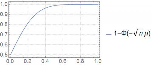
Let’s plot this power function, for [math]n=20[/math], as a function of the parameter of interest, [math]\mu[/math]:
Under the null hypothesis, [math]\mu=0[/math]. In this case, the probability of committing a type 1 error is [math]50\%[/math]. This means that if we repeated this exact experiment many times with [math]\mu=0[/math], and drew multiple values of [math]\overline{x}[/math] each time, our rule would have rejected the null hypothesis approximately 50% of the time.
Is this surprising? The magical 50% figure is a consequence of the chosen test statistic and the cutoff of zero of our admittedly arbitrary rule. The random variable of interest in our test (i.e., our test statistic) is the sample mean. We obtained this result because a [math]N\left(0,1\right)[/math] produces sample means (each calculated with [math]n=20[/math]) above zero 50% of the time. Whether this rejection rate of the null hypothesis is appropriate depends on the application.
What does the power function tell us?
It tells us the probability of rejecting [math]H_{0}[/math] when [math]\mu=0[/math], according to our rule. At [math]H_{1}[/math] ([math]\mu\gt 0[/math]), it gives us one minus the probability of committing a type 2 error. In other words, at [math]\mu\gt 0[/math], it tells us the probability of accepting the alternative hypothesis when it was indeed correct, for each specific value of [math]\mu[/math].
We would like to produce a power function that equals zero at [math]\mu=0[/math], and equals 1 at [math]\mu\gt 1[/math]. However, as long as [math]\overline{X}[/math] is uncertain, we cannot ensure this.
Intuitively, we want to minimize the power function at the null set, and maximize it at the alternative set.
